Airborne Wind Energy - Tutorials AE3513

Updated: 22 Oct 2026

In this tutorial you will estimate the power production of a pumping-cycle airborne wind energy (AWE) system for a given wind speed time series.

A pumping kite power system consists of a kite connected by a tether to a drum and generator on the ground. The cycle has two phases:

Reel-out (traction phase): the kite flies fast crosswind and pulls the tether out. The drum drives the generator and produces power.
Reel-in (retraction phase): the kite is depowered and reeled back in, using a small fraction of the energy that was produced.

The net cycle power is the energy produced during reel-out minus the energy used for reel-in, averaged over the whole cycle.

After this tutorial you will be able to:

compute the power curve of a pumping AWE system, which gives the cycle power as a function of wind speed;
explain the three wind speed regimes of the power curve;
generate a dummy wind speed time series;
convert the time series into a power time series and calculate the energy yield and the capacity factor.

The power curve model is adapted from the awecourse/resources repository (MIT license, R. Schmehl), which follows the control strategy of Luchsinger Luchsinger (2013) and the system characterisation of Van der Vlugt et al. Vlugt et al. (2013).

1. System properties¶

The default values describe a small kite power system with a 16.7 m $^2$ soft kite, a 5 kN nominal tether force and a 20 kW generator (SI units).

import numpy as np
import matplotlib.pyplot as plt
import ipywidgets as widgets
from ipywidgets import interact
from scipy import optimize as op

system = dict(
    rho=1.225,            # air density [kg/m^3]
    A=16.7,               # kite planform area [m^2]
    CL_out=1.0,           # kite lift coefficient, reel-out [-]
    CD_kite_out=0.2,      # kite drag coefficient, reel-out [-]
    CL_in=0.14,           # kite lift coefficient, reel-in [-]
    CD_in=0.07,           # kite drag coefficient, reel-in [-]
    F_nom=5000.0,         # nominal tether force [N]
    CD_tether=1.1,        # tether drag coefficient [-]
    d_tether=0.00484,     # tether diameter [m]
    l_max=375.0,          # maximum tether length [m]
    l_min=200.0,          # minimum tether length [m]
    P_gen=20000.0,        # nominal generator power [W]
    beta_out_deg=25.0,    # elevation angle during reel-out [deg]
    v_reel_min=-8.0,      # maximum reel-in speed [m/s]
    v_reel_max=8.0,       # maximum reel-out speed [m/s]
)

# Plot style: accent colour palette, no grid
from cycler import cycler
plt.rcParams.update({
    'axes.prop_cycle': cycler(color=['#017188', '#EC6842', '#00A6D6', '#6CC24A', '#A50034']),
    'axes.grid': False,
    'axes.spines.top': False,
    'axes.spines.right': False,
    'lines.linewidth': 2,
})

2. Power curve model¶

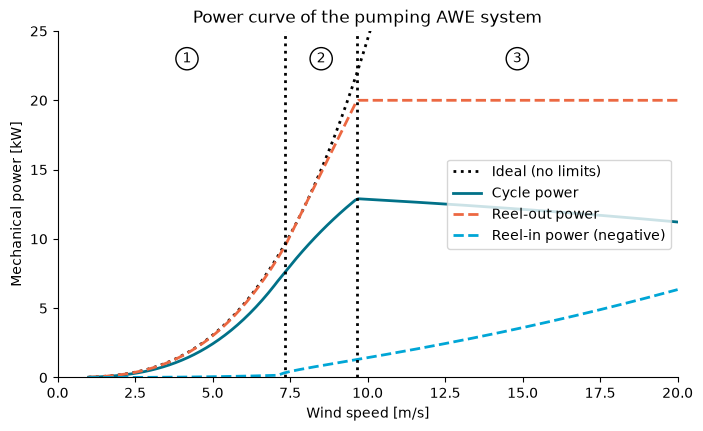
For every wind speed $v_w$ the model finds the reeling factors $f_\mathrm{o}$ and $f_\mathrm{i}$ (reeling speed divided by wind speed, during reel-out and reel-in) that maximise the cycle power. Three wind speed regimes appear:

Low wind: no limit is active. The system follows the optimum, so the power grows with $v_w^3$ .
Tether force limited (above $v_\mathrm{n,F}$ ): the tether force has reached its nominal value. The reel-out speed is increased to keep the force constant.
Generator power limited (above $v_\mathrm{n,P}$ ): the generator is at its rated power. The kite is depowered to keep the power constant.

The function below is a direct adaptation of powercurve_const_LoD_in.py from the course repository. The script was restructured into a function, with the same equations. In this version the reel-in phase uses a constant lift-to-drag ratio, so the reel-in elevation angle follows from the wind speed. You do not need to read the details to continue.

def pumping_power_curve(wind_speed, rho, A, CL_out, CD_kite_out, CL_in, CD_in,
                        F_nom, CD_tether, d_tether, l_max, l_min, P_gen,
                        beta_out_deg, v_reel_min, v_reel_max, f_eps=1e-4):
    """Cycle power [W] of a pumping AWE system for a uniformly spaced wind speed array [m/s]."""
    dv = wind_speed[1] - wind_speed[0]

    # Derived properties
    CD_out = CD_kite_out + 0.25 * CD_tether * d_tether * 0.5 * (l_min + l_max) / A
    E2out = (CL_out / CD_out) ** 2
    E2in = (CL_in / CD_in) ** 2
    cos_b = np.cos(np.radians(beta_out_deg))
    ff_out0 = CL_out * np.sqrt(1 + 1 / E2out) * (1 + E2out)
    ff_in = CL_in * np.sqrt(1 + 1 / E2in)
    p_factor_ideal = ff_out0 * cos_b ** 3 * 4 / 27

    def reel_in_term(f_in):
        return (np.sqrt(1 + E2in * (1 - f_in ** 2)) - f_in) ** 2 / (1 + E2in)

    # Objective functions (negative normalised cycle power) of the three regimes
    def obj1(x):
        f_out, f_in = x
        return -((cos_b - f_out) ** 2 - (ff_in / ff_out0) * reel_in_term(f_in)) \
               * (f_in * f_out) / (f_in - f_out)

    def obj2(x, mu_F, f_nF):
        f_in = x[0]
        b = (mu_F - 1) * cos_b + f_nF
        return -(((cos_b - f_nF) / mu_F) ** 2 - (ff_in / ff_out0) * reel_in_term(f_in)) \
               * f_in * b / (mu_F * f_in - b)

    def obj3(x, mu_P, f_nP, ff_out):
        f_in = x[0]
        return -((cos_b - f_nP / mu_P) ** 2 - (ff_in / ff_out) * reel_in_term(f_in)) \
               * f_in * f_nP / (mu_P * f_in - f_nP)

    def bisect(func, v_a, v_b, target, eps=0.1, nmax=100):
        for _ in range(nmax):
            v = 0.5 * (v_a + v_b)
            value = func(v)
            if value > target:
                v_b = v
            else:
                v_a = v
            if abs(value - target) < eps:
                break
        return v

    regime = 1
    v_nF = v_nP = np.nan
    out = {k: [] for k in ('cycle', 'out', 'in', 'ideal', 'f_out', 'f_in')}

    for v_w in wind_speed:
        q = 0.5 * rho * v_w ** 2          # dynamic pressure
        P_w = q * v_w                      # wind power density
        f_min = max(v_reel_min / v_w, -np.sqrt(1 + 1 / E2in))
        f_max = min(v_reel_max / v_w, 1.0)
        ff_out = ff_out0

        if regime == 1:
            res = op.minimize(obj1, (f_eps, -f_eps), method='SLSQP',
                              bounds=((f_eps, f_max), (f_min, -f_eps)))
            f_out, f_in = res['x']
            p_c = -obj1([f_out, f_in])
            if q * A * ff_out * (cos_b - f_out) ** 2 > F_nom:
                regime = 2
                c = 0.5 * rho * A * ff_out * (cos_b - f_out) ** 2
                v_nF = bisect(lambda v: c * v ** 2, v_w - dv, v_w, F_nom)
                f_nF = f_out

        if regime == 2:
            mu_F = v_w / v_nF
            res = op.minimize(obj2, (-f_eps), args=(mu_F, f_nF), method='SLSQP',
                              bounds=((f_min, -f_eps),))
            f_out = (cos_b * (mu_F - 1) + f_nF) / mu_F
            f_in = res['x'][0]
            p_c = -obj2([f_in], mu_F, f_nF)
            if q * A * ff_out * (cos_b - f_out) ** 2 * v_w * f_out > P_gen:
                regime = 3
                c = 0.5 * rho * A * ff_out

                def power_out(v):
                    mu = v / v_nF
                    f = (cos_b * (mu - 1) + f_nF) / mu
                    return c * (cos_b - f) ** 2 * v ** 3 * f

                v_nP = bisect(power_out, v_w - dv, v_w, P_gen)
                mu = v_nP / v_nF
                f_nP = (cos_b * (mu - 1) + f_nF) / mu

        if regime == 3:
            mu_P = v_w / v_nP
            f_out = f_nP / mu_P
            # Depower the kite to respect the tether force limit
            ff_out = F_nom / (q * A * (cos_b - f_out) ** 2)
            res = op.minimize(obj3, (-f_eps), args=(mu_P, f_nP, ff_out), method='SLSQP',
                              bounds=((f_min, -f_eps),))
            f_in = res['x'][0]
            p_c = -obj3([f_in], mu_P, f_nP, ff_out)

        F_out = q * A * ff_out * (cos_b - f_out) ** 2
        F_in = q * A * ff_in * reel_in_term(f_in)
        out['out'].append(F_out * v_w * f_out)
        out['in'].append(F_in * v_w * f_in)
        out['cycle'].append(p_c * ff_out * A * P_w)
        out['ideal'].append(p_factor_ideal * A * P_w)
        out['f_out'].append(f_out)
        out['f_in'].append(f_in)

    result = {k: np.array(v) for k, v in out.items()}
    result.update(wind_speed=np.asarray(wind_speed), v_nF=v_nF, v_nP=v_nP)
    return result

Compute and plot the power curve¶

We compute the curve for wind speeds from 1 to 20 m/s in steps of 0.1 m/s. This takes a few seconds.

v_grid = np.arange(1.0, 20.0 + 0.05, 0.1)
with np.errstate(invalid='ignore'):  # the optimiser probes points outside the valid range
    curve = pumping_power_curve(v_grid, **system)

rated_power = curve['cycle'].max()
print(f"Rated cycle power: {rated_power / 1e3:.1f} kW")
print(f"Tether force limit reached at v_n,F = {curve['v_nF']:.1f} m/s")
print(f"Generator power limit reached at v_n,P = {curve['v_nP']:.1f} m/s")

fig, ax = plt.subplots(figsize=(8, 4.5))
ax.plot(v_grid, curve['ideal'] / 1e3, 'k:', label='Ideal (no limits)')
ax.plot(v_grid, curve['cycle'] / 1e3, label='Cycle power')
ax.plot(v_grid, curve['out'] / 1e3, linestyle='--', label='Reel-out power')
ax.plot(v_grid, -curve['in'] / 1e3, linestyle='--', label='Reel-in power (negative)')
ax.axvline(curve['v_nF'], color='k', linestyle=':')
ax.axvline(curve['v_nP'], color='k', linestyle=':')
for x, label in [(0.5 * (v_grid[0] + curve['v_nF']), '1'),
                 (0.5 * (curve['v_nF'] + curve['v_nP']), '2'),
                 (0.5 * (curve['v_nP'] + v_grid[-1]), '3')]:
    ax.annotate(label, (x, 23), ha='center', va='center',
                bbox=dict(boxstyle='circle', fc='white', ec='k'))
ax.set_xlim(0, 20)
ax.set_ylim(0, 25)
ax.set_xlabel('Wind speed [m/s]')
ax.set_ylabel('Mechanical power [kW]')
ax.set_title('Power curve of the pumping AWE system')
ax.legend(loc='center right')
plt.show()

Rated cycle power: 12.9 kW
Tether force limit reached at v_n,F = 7.3 m/s
Generator power limit reached at v_n,P = 9.7 m/s

3. A dummy wind speed time series¶

We now need a wind speed time series. Instead of measured data, we generate a synthetic one made of three parts:

a mean wind speed;
a daily cycle, with the strongest wind in the afternoon;
correlated random fluctuations (an AR(1) process), so that consecutive values are similar.

The random generator is seeded, so everyone gets the same series.

def make_wind_series(mean=8.0, daily_amplitude=2.0, fluctuation=1.5,
                     n_days=3, dt_min=10, seed=1):
    """Return time [h] and wind speed [m/s] with a time step of dt_min minutes."""
    rng = np.random.default_rng(seed)
    t = np.arange(0, n_days * 24, dt_min / 60)

    # Daily cycle with maximum at 15:00
    daily = daily_amplitude * np.cos(2 * np.pi * (t - 15) / 24)

    # AR(1) fluctuations with a standard deviation of `fluctuation`
    phi = 0.95
    noise = np.zeros_like(t)
    for i in range(1, len(t)):
        noise[i] = phi * noise[i - 1] + rng.normal(0, fluctuation * np.sqrt(1 - phi ** 2))

    return t, np.clip(mean + daily + noise, 0, None)


dt_h = 10 / 60  # time step in hours
t, wind = make_wind_series()

fig, ax = plt.subplots(figsize=(9, 3.5))
ax.plot(t, wind)
ax.set_xlabel('Time [h]')
ax.set_ylabel('Wind speed [m/s]')
ax.set_title('Dummy wind speed time series')
plt.show()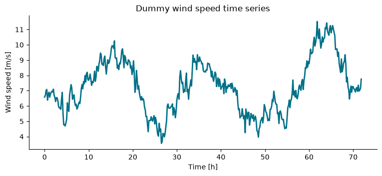

4. From wind speed to power¶

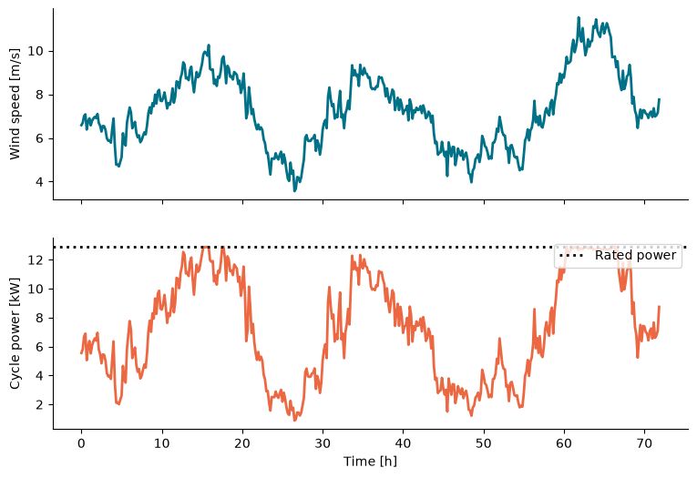
The power curve gives the cycle power for every wind speed. We apply it to each point of the time series using interpolation. Two rules are added:

if the curve gives zero or negative power (too little wind for a net gain), the system produces nothing;
above the highest wind speed of the curve (20 m/s) the system is shut down for safety.

The energy is the sum of power times the time step, and the capacity factor is the produced energy divided by the energy at rated power over the same period.

def power_from_wind(wind, curve):
    """Cycle power [W] for a wind speed time series."""
    power = np.interp(wind, curve['wind_speed'], curve['cycle'], left=0.0, right=0.0)
    return np.clip(power, 0, None)


power = power_from_wind(wind, curve)

energy_kwh = power.sum() * dt_h / 1e3
capacity_factor = power.mean() / rated_power
print(f"Mean wind speed:  {wind.mean():.1f} m/s")
print(f"Mean power:       {power.mean() / 1e3:.1f} kW")
print(f"Energy produced:  {energy_kwh:.0f} kWh in {t[-1] + dt_h:.0f} h")
print(f"Capacity factor:  {capacity_factor:.2f}")

fig, (ax1, ax2) = plt.subplots(2, 1, figsize=(9, 6), sharex=True)
ax1.plot(t, wind)
ax1.set_ylabel('Wind speed [m/s]')
ax2.plot(t, power / 1e3, color='C1')
ax2.axhline(rated_power / 1e3, color='k', linestyle=':', label='Rated power')
ax2.set_xlabel('Time [h]')
ax2.set_ylabel('Cycle power [kW]')
ax2.legend(loc='upper right')
plt.show()

Mean wind speed:  7.3 m/s
Mean power:       7.3 kW
Energy produced:  524 kWh in 72 h
Capacity factor:  0.56

The scatter plot below shows that every point of the time series lies on the power curve. Compare the wind speeds in the series with $v_\mathrm{n,F}$ and $v_\mathrm{n,P}$ : how often is the system in each regime?

fig, ax = plt.subplots(figsize=(7, 4.5))
ax.plot(v_grid, curve['cycle'] / 1e3, label='Power curve')
ax.plot(wind, power / 1e3, 'o', color='C1', markersize=3, alpha=0.4, label='Time series')
ax.set_xlabel('Wind speed [m/s]')
ax.set_ylabel('Cycle power [kW]')
ax.set_xlim(0, 20)
ax.legend()
plt.show()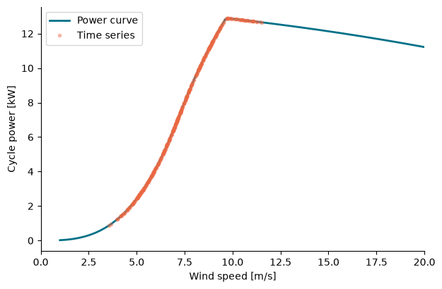

5. Interactive: effect of the wind conditions¶

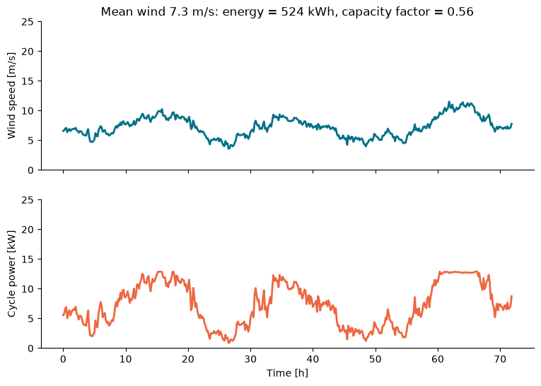
Use the sliders to change the mean wind speed and the size of the fluctuations. The power curve is reused, so the result updates immediately. How strongly does the energy yield depend on the mean wind speed?

def update(mean_wind, fluctuation):
    t, wind = make_wind_series(mean=mean_wind, fluctuation=fluctuation)
    power = power_from_wind(wind, curve)
    energy = power.sum() * dt_h / 1e3
    cf = power.mean() / rated_power

    fig, (ax1, ax2) = plt.subplots(2, 1, figsize=(9, 6), sharex=True)
    ax1.plot(t, wind)
    ax1.set_ylabel('Wind speed [m/s]')
    ax1.set_ylim(0, 25)
    ax2.plot(t, power / 1e3, color='C1')
    ax2.set_xlabel('Time [h]')
    ax2.set_ylabel('Cycle power [kW]')
    ax2.set_ylim(0, 25)
    ax1.set_title(f'Mean wind {wind.mean():.1f} m/s: energy = {energy:.0f} kWh, capacity factor = {cf:.2f}')
    plt.show()


interact(
    update,
    mean_wind=widgets.FloatSlider(
        min=3, max=14, step=0.5, value=8, description='Mean wind [m/s]',
        continuous_update=False, style={'description_width': 'initial'},
    ),
    fluctuation=widgets.FloatSlider(
        min=0, max=3, step=0.25, value=1.5, description='Fluctuation [m/s]',
        continuous_update=False, style={'description_width': 'initial'},
    ),
);

References¶

Luchsinger, R. H. (2013). Pumping Cycle Kite Power. In U. Ahrens, M. Diehl, & R. Schmehl (Eds.), Airborne Wind Energy (pp. 47–64). Springer. 10.1007/978-3-642-39965-7_3
Van der Vlugt, R., Peschel, J., & Schmehl, R. (2013). Design and Experimental Characterization of a Pumping Kite Power System. In U. Ahrens, M. Diehl, & R. Schmehl (Eds.), Airborne Wind Energy (pp. 403–425). Springer. 10.1007/978-3-642-39965-7_23