Storage System Dispatch - Tutorials AE3513

Updated: 22 Oct 2026

A variable power source (wind, solar, airborne wind energy) rarely matches a constant demand. An energy storage can smooth the output: it absorbs the surplus when production is high and releases energy when production is low.

After this tutorial you will be able to:

define a storage system and a dummy power time series;
implement a rule-based dispatch that targets a minimum (baseload) power;
check the result with an energy balance;
explain how the baseload and the storage size influence how often the baseload is met.

1. Storage system and power time series¶

The storage is described by its energy capacity, its power capacity and its round-trip efficiency. The efficiency is applied when charging: charging with $P$ for a time $\Delta t$ stores $P \Delta t \eta$ , while discharging is lossless.

The power series is dummy data: a daily cycle plus random fluctuations, with a time step of 1 hour.

import numpy as np
import matplotlib.pyplot as plt
from ipywidgets import interact, FloatSlider

# Plot style: accent colour palette, no grid
from cycler import cycler
plt.rcParams.update({
    'axes.prop_cycle': cycler(color=['#017188', '#EC6842', '#00A6D6', '#6CC24A', '#A50034']),
    'axes.grid': False,
    'axes.spines.top': False,
    'axes.spines.right': False,
    'lines.linewidth': 2,
})

storage = dict(
    e_cap=100,  # Energy capacity [MWh]
    p_cap=20,  # Power capacity [MW]
    efficiency=0.9,  # Round-trip efficiency [-]
)

dt = 1  # Time step [h]
n = 72  # Number of time steps [-]
time = np.arange(n) * dt

rng = np.random.default_rng(seed=1)
power = 30 + 15 * np.sin(2 * np.pi * (time - 6) / 24) + rng.normal(0, 6, n)
power = np.clip(power, 0, None)  # Power produced [MW]

fig, ax = plt.subplots(figsize=(9, 3))
ax.plot(time, power)
ax.set_xlabel("Time [h]")
ax.set_ylabel("Power [MW]")
ax.set_title(f"Dummy power series (mean {power.mean():.1f} MW)")
plt.show()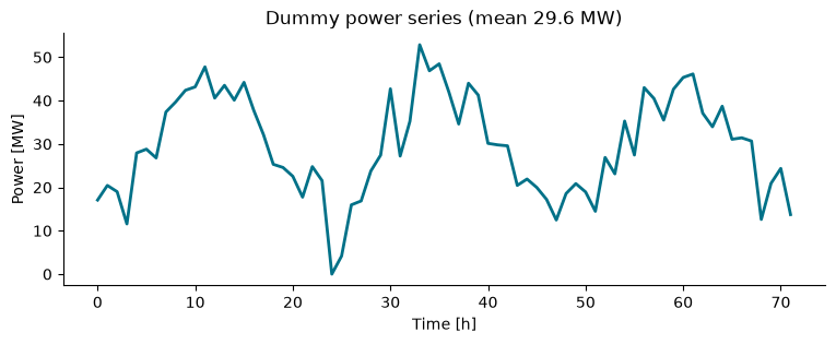

2. Rule-based dispatch for a baseload¶

The objective is to deliver at least a baseload power $P_\mathrm{min}$ :

if the power produced is above $P_\mathrm{min}$ , the surplus charges the storage, limited by the power capacity and the free energy capacity;
if the power produced is below $P_\mathrm{min}$ , the storage discharges to cover the shortfall, limited by the power capacity and the energy stored.

Sign convention: the storage power stor_p is negative when charging and positive when discharging.

This code is adapted from shipp.kernel.os_rule_based in the SHIPP software (Iori (2025)).

def dispatch_baseload(
    power, e_cap, p_cap, efficiency, p_min, n, e_start=0.0, dt=1.0
):
    """Dispatch a storage to supply a minimum baseload power.

    The storage is charged with the power above p_min and discharged when the
    power is below p_min. The round-trip efficiency is applied when charging.

    Args:
        power: Power produced at each time step [MW], length n.
        e_cap: Energy capacity of the storage [MWh].
        p_cap: Power capacity of the storage [MW].
        efficiency: Round-trip efficiency [-].
        p_min: Baseload power to deliver [MW].
        n: Number of time steps.
        e_start: Initial stored energy [MWh].
        dt: Time step [h].

    Returns:
        stor_e: Stored energy at each time step [MWh], length n + 1.
        stor_p: Storage power [MW], length n. Negative when charging.
    """
    stor_e = np.zeros(n + 1)
    stor_e[0] = e_start
    stor_p = np.zeros(n)

    for t in range(n):
        if power[t] >= p_min:
            # Charge: limited by power capacity, free capacity and surplus
            surplus = power[t] - p_min
            stor_p[t] = -min(p_cap, (e_cap - stor_e[t]) / dt / efficiency, surplus)
            stor_e[t + 1] = stor_e[t] - dt * stor_p[t] * efficiency
        else:
            # Discharge: limited by power capacity, stored energy and shortfall
            missing = p_min - power[t]
            stor_p[t] = min(p_cap, stor_e[t] / dt, missing)
            stor_e[t + 1] = stor_e[t] - dt * stor_p[t]

    return stor_e, stor_p

3. Results¶

We choose a baseload and compute the power delivered, which is the sum of the power produced and the storage power.

p_min = 28  # Baseload [MW]

stor_e, stor_p = dispatch_baseload(power, p_min=p_min, n=n, dt=dt, **storage)
delivered = power + stor_p

hours_ok = np.sum(delivered >= p_min - 1e-9) * dt
print(f"Baseload met during {hours_ok:.0f} of {n * dt} hours ({100 * hours_ok / (n * dt):.0f} %)")

fig, axs = plt.subplots(3, 1, figsize=(9, 8), sharex=True)
axs[0].plot(time, power, label="Produced")
axs[0].plot(time, delivered, label="Delivered")
axs[0].axhline(p_min, color="k", linestyle="--", label="Baseload")
axs[0].set_ylabel("Power [MW]")
axs[0].legend()
axs[1].plot(time, stor_p)
axs[1].set_ylabel("Storage power [MW]\n(<0: charging)")
axs[2].plot(time, stor_e[:-1])
axs[2].set_ylabel("Stored energy [MWh]")
axs[2].set_xlabel("Time [h]")
plt.show()

Baseload met during 64 of 72 hours (89 %)

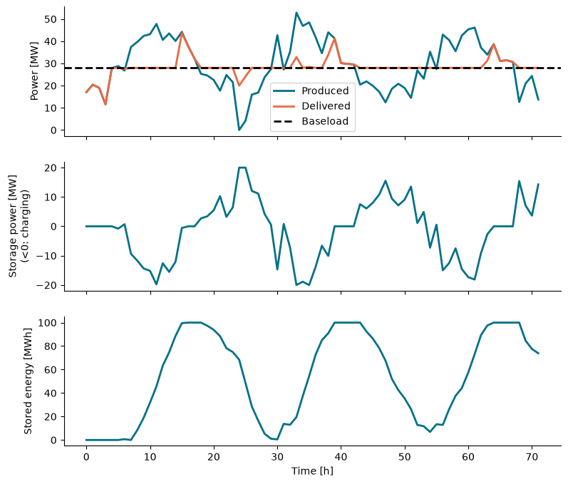
The storage starts empty, so the baseload cannot be met in the first low-power period. Later, the stored energy bridges the dips.

A quick check of the energy balance: the energy delivered equals the energy produced minus the losses in the storage and the change in stored energy.

charged = -stor_p[stor_p < 0].sum() * dt
losses = charged * (1 - storage["efficiency"])
print(f"Produced:  {power.sum() * dt:8.1f} MWh")
print(f"Delivered: {delivered.sum() * dt:8.1f} MWh")
print(f"Losses:    {losses:8.1f} MWh")
print(f"Stored:    {stor_e[-1] - stor_e[0]:8.1f} MWh")
print(f"Balance:   {power.sum() * dt - delivered.sum() * dt - losses - (stor_e[-1] - stor_e[0]):8.1e} MWh")

Produced:    2134.7 MWh
Delivered:   2042.3 MWh
Losses:        32.7 MWh
Stored:        59.6 MWh
Balance:    2.3e-13 MWh

4. Interactive: effect of the baseload and the storage size¶

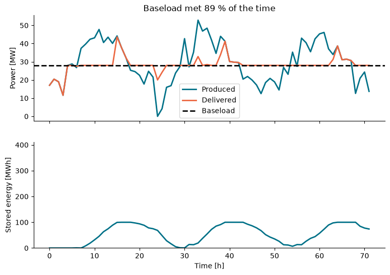
Use the sliders to change the baseload and the energy capacity of the storage. A higher baseload is met less often, and a larger storage helps to bridge longer low-power periods.

def update(p_min=28.0, e_cap=100.0):
    stor_e, stor_p = dispatch_baseload(
        power, e_cap, storage["p_cap"], storage["efficiency"], p_min, n, dt=dt
    )
    delivered = power + stor_p
    share = 100 * np.sum(delivered >= p_min - 1e-9) / n

    fig, axs = plt.subplots(2, 1, figsize=(9, 6), sharex=True)
    axs[0].plot(time, power, label="Produced")
    axs[0].plot(time, delivered, label="Delivered")
    axs[0].axhline(p_min, color="k", linestyle="--", label="Baseload")
    axs[0].set_ylabel("Power [MW]")
    axs[0].set_title(f"Baseload met {share:.0f} % of the time")
    axs[0].legend()
    axs[1].plot(time, stor_e[:-1])
    axs[1].set_ylim(0, 410)
    axs[1].set_ylabel("Stored energy [MWh]")
    axs[1].set_xlabel("Time [h]")
    plt.show()


interact(
    update,
    p_min=FloatSlider(value=28, min=10, max=40, step=1, description="Baseload [MW]", style={"description_width": "initial"}),
    e_cap=FloatSlider(value=100, min=0, max=400, step=10, description="E cap [MWh]", style={"description_width": "initial"}),
);

References¶

Iori, J. (2025). SHIPP - A design optimization software for hybrid power plants. 4TU.ResearchData. 10.4121/2ee36148-369f-4e1f-b770-c86752d7dca4