Wind Farm Simulation with FLORIS

Updated: 22 Oct 2026

In this tutorial you will use FLORIS, an open-source wind farm simulation framework (National Laboratory of the Rockies (2025)), to see how turbines affect each other through their wakes. A turbine extracts energy from the wind, so the air behind it is slower and more turbulent. Downstream turbines therefore produce less power than turbines in undisturbed flow.

After this tutorial you will be able to:

create a FLORIS model and define a wind farm layout;
set the inflow conditions (wind speed, wind direction, turbulence intensity);
run the simulation and read the power of each turbine and of the whole farm;
visualise the wake flow field and explain how the wind direction changes the farm power.

This tutorial is adapted from the FLORIS examples 001 and 002.

1. Set up the model¶

The FlorisModel class is the entry point for most FLORIS usage. Initialising it with "defaults" loads default wake model and atmospheric settings. We then define the IEA 10 MW reference turbine (198 m rotor diameter, 119 m hub height) from its power curve and thrust coefficient curve, taken from the IEA Wind 740-10-MW reference offshore wind plants (Kainz et al. (2024)). The curves are listed in the first code cell below. We place 8 turbines on an irregular layout, given as lists of $x$ and $y$ coordinates in metres.

The wind is assumed uniform over the height of the rotor (no wind shear), so that the result can be compared with the PyWake tutorial.

import numpy as np

# Power and thrust coefficient curves of the IEA 10 MW reference turbine, from the
# IEA Wind 740-10-MW Reference Offshore Wind Plants (file IEA37_10MW_turbine.yaml)
turbine_ws = np.array([
    4.000, 4.515, 5.001, 5.457, 5.883, 6.278, 6.640, 6.968,
    7.263, 7.523, 7.748, 7.938, 8.091, 8.208, 8.288, 8.331,
    8.337, 8.368, 8.436, 8.540, 8.681, 8.859, 9.072, 9.320,
    9.604, 9.921, 10.272, 10.656, 10.758, 11.518, 11.994, 12.499,
    13.032, 13.592, 14.177, 14.786, 15.418, 16.070, 16.743, 17.434,
    18.142, 18.865, 19.602, 20.351, 21.110, 21.877, 22.652, 23.432,
    24.215, 25.000,
])  # Wind speed [m/s]

turbine_power = np.array([
    387.5, 644.7, 938.0, 1257.9, 1604.1, 1969.5, 2340.1, 2708.6,
    3067.1, 3408.7, 3723.7, 4003.4, 4239.6, 4425.8, 4556.6, 4628.1,
    4638.4, 4690.0, 4804.9, 4985.7, 5236.9, 5564.4, 5975.8, 6480.5,
    7089.7, 7816.4, 8690.6, 9716.7, 10000.0, 10000.0, 10000.0, 10000.0,
    10000.0, 10000.0, 10000.0, 10000.0, 10000.0, 10000.0, 10000.0, 10000.0,
    10000.0, 10000.0, 10000.0, 10000.0, 10000.0, 10000.0, 10000.0, 10000.0,
    10000.0, 10000.0,
])  # Power [kW]

turbine_ct = np.array([
    0.7701, 0.7763, 0.7824, 0.7820, 0.7802, 0.7772, 0.7719, 0.7768,
    0.7768, 0.7768, 0.7768, 0.7768, 0.7768, 0.7768, 0.7768, 0.7768,
    0.7768, 0.7768, 0.7768, 0.7768, 0.7768, 0.7768, 0.7768, 0.7768,
    0.7768, 0.7768, 0.7675, 0.7651, 0.7587, 0.5056, 0.4310, 0.3708,
    0.3209, 0.2788, 0.2432, 0.2128, 0.1868, 0.1645, 0.1454, 0.1289,
    0.1147, 0.1024, 0.0918, 0.0825, 0.0745, 0.0675, 0.0613, 0.0559,
    0.0512, 0.0470,
])  # Thrust coefficient [-]

rotor_diameter = 198.0  # [m]
hub_height = 119.0  # [m]
cut_in, cut_out = 4.0, 25.0  # Cut-in and cut-out wind speed [m/s]

import matplotlib.pyplot as plt
import numpy as np
import ipywidgets as widgets
from ipywidgets import interact

import floris.layout_visualization as layoutviz
from floris import FlorisModel
from floris.flow_visualization import visualize_cut_plane

fmodel = FlorisModel("defaults")

# Turbine positions [m]
layout_x = [0, 500, 0, 128, 1000, 900, 1500, 1250]
layout_y = [0, 300, 750, 1400, 0, 567, 888, 1450]
# Turbine definition: power in kW, thrust coefficient and wind speed tables
turbine = {
    "turbine_type": "iea_10MW_rowp",
    "hub_height": hub_height,
    "rotor_diameter": rotor_diameter,
    "TSR": 8.0,  # Not used by the simple operation model
    "operation_model": "simple",
    "power_thrust_table": {
        "ref_air_density": 1.225,
        "ref_tilt": 5.0,
        "wind_speed": turbine_ws.tolist(),
        "power": turbine_power.tolist(),
        "thrust_coefficient": turbine_ct.tolist(),
    },
}

fmodel.set(
    layout_x=layout_x,
    layout_y=layout_y,
    turbine_type=[turbine],
    reference_wind_height=hub_height,  # The wind speed is defined at hub height
    wind_shear=0.0,  # Uniform wind over the height of the rotor
)

# Plot style: accent colour palette, no grid
from cycler import cycler
plt.rcParams.update({
    'axes.prop_cycle': cycler(color=['#017188', '#EC6842', '#00A6D6', '#6CC24A', '#A50034']),
    'axes.grid': False,
    'axes.spines.top': False,
    'axes.spines.right': False,
    'lines.linewidth': 2,
})

Let’s check the layout. The numbers are the turbine indices, which we will use later to read the power per turbine.

fig, ax = plt.subplots()
layoutviz.plot_turbine_points(fmodel, ax=ax)
layoutviz.plot_turbine_labels(fmodel, ax=ax)
ax.set_title("Wind farm layout")
ax.set_xlabel("x [m]")
ax.set_ylabel("y [m]")
ax.set_aspect("equal")
plt.show()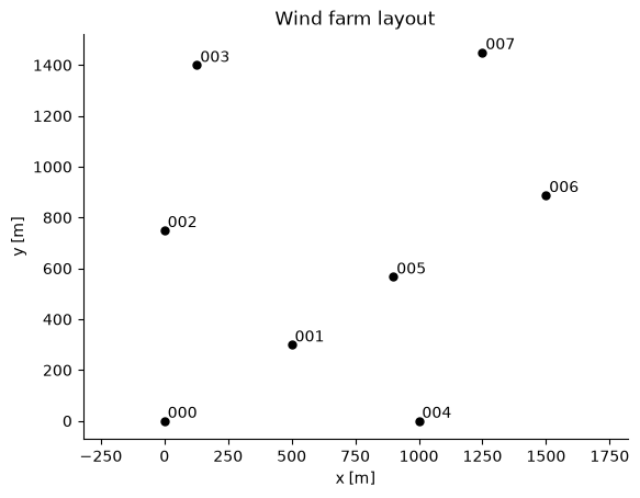

The power curve gives the power of one turbine as a function of the wind speed. Below the cut-in wind speed (4 m/s) the turbine does not produce power. Above the rated wind speed the power stays at the rated power of 10 MW. The thrust coefficient $C_T$ describes how strongly the rotor slows down the wind, and so how strong the wake is.

fig, axs = plt.subplots(1, 2, figsize=(9, 3.5))
axs[0].plot(turbine_ws, turbine_power / 1e3)
axs[0].set_ylabel("Power [MW]")
axs[1].plot(turbine_ws, turbine_ct, color="C1")
axs[1].set_ylabel("Thrust coefficient [-]")
for ax in axs:
    ax.axvline(cut_in, color="k", linestyle=":")
    ax.axvline(cut_out, color="k", linestyle=":")
    ax.set_xlabel("Wind speed [m/s]")
    ax.set_xlim([0, 26])
fig.suptitle("IEA 10 MW reference turbine (dotted: cut-in and cut-out)")
plt.tight_layout()
plt.show()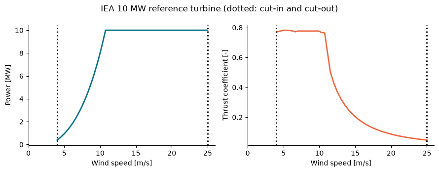

2. Run a single wind condition¶

The inflow is defined by three quantities:

the wind speed at hub height [m/s];
the wind direction [deg], defined as the direction the wind comes from (meteorological convention): $270^\circ$ is a westerly wind, blowing towards the east (+ $x$ ), and $0^\circ$ is a northerly wind, blowing towards the south;
the turbulence intensity [-], which controls how fast the wake recovers.

Each is given as a list: FLORIS can evaluate many conditions at once (one per list entry). Here we use a single condition.

fmodel.set(wind_speeds=[8.0], wind_directions=[270.0], turbulence_intensities=[0.06])
fmodel.run()

# Arrays have shape (number of conditions, number of turbines); power is in W
turbine_powers = fmodel.get_turbine_powers() / 1e6
farm_power = fmodel.get_farm_power() / 1e6

for i, p in enumerate(turbine_powers[0]):
    print(f"Turbine {i}: {p:.2f} MW")
print(f"Farm power: {farm_power[0]:.2f} MW")

Turbine 0: 4.10 MW
Turbine 1: 4.10 MW
Turbine 2: 4.10 MW
Turbine 3: 4.10 MW
Turbine 4: 1.05 MW
Turbine 5: 3.75 MW
Turbine 6: 3.16 MW
Turbine 7: 1.62 MW
Farm power: 25.98 MW

3. Visualise the flow field¶

To visualise the wakes we ask FLORIS to compute the wind speed on a horizontal plane at hub height (119 m). The resolution is kept low so that the calculation is fast.

horizontal_plane = fmodel.calculate_horizontal_plane(
    x_resolution=100, y_resolution=100, height=hub_height
)

fig, ax = plt.subplots()
visualize_cut_plane(
    horizontal_plane,
    ax=ax,
    label_contours=False,
    title="Wind speed at hub height (wind from the west)",
    cmap="bone",
)
layoutviz.plot_turbine_rotors(fmodel, ax=ax)
layoutviz.plot_turbine_labels(fmodel, ax=ax)
ax.set_xlabel("x [m]")
ax.set_ylabel("y [m]")
plt.show()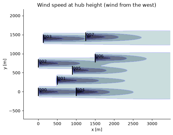

4. Interactive: effect of the wind direction¶

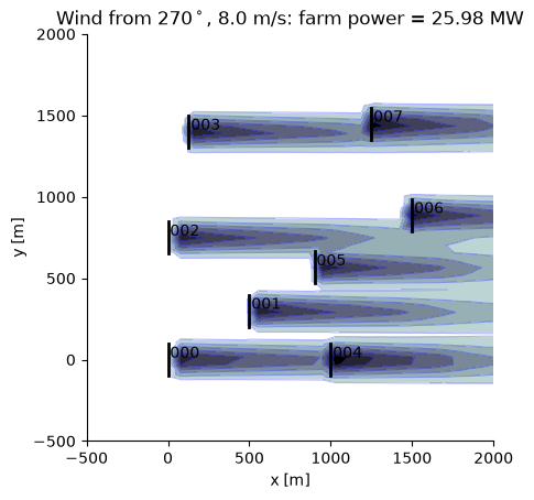
Use the sliders to change the wind direction and the wind speed. The farm power is shown in the plot title. The calculation is only updated when you release the slider.

def update(wind_direction, wind_speed):
    fmodel.set(
        wind_speeds=[wind_speed],
        wind_directions=[wind_direction],
        turbulence_intensities=[0.06],
    )
    fmodel.run()
    farm_power = fmodel.get_farm_power()[0] / 1e6

    horizontal_plane = fmodel.calculate_horizontal_plane(
        x_resolution=50, y_resolution=50, height=hub_height
    )

    fig, ax = plt.subplots()
    visualize_cut_plane(
        horizontal_plane,
        ax=ax,
        label_contours=False,
        title=f"Wind from {wind_direction:.0f}$^\\circ$, {wind_speed:.1f} m/s: farm power = {farm_power:.2f} MW",
        cmap="bone",
    )
    layoutviz.plot_turbine_rotors(fmodel, ax=ax)
    layoutviz.plot_turbine_labels(fmodel, ax=ax)
    ax.set_xlabel("x [m]")
    ax.set_ylabel("y [m]")
    ax.set_xlim([-500, 2000])
    ax.set_ylim([-500, 2000])
    ax.set_aspect("equal", adjustable="box")
    plt.show()


interact(
    update,
    wind_direction=widgets.FloatSlider(
        min=0, max=360, step=30, value=270, description="Direction [deg]",
        continuous_update=False, style={"description_width": "initial"},
    ),
    wind_speed=widgets.FloatSlider(
        min=4, max=14, step=1, value=8, description="Speed [m/s]",
        continuous_update=False, style={"description_width": "initial"},
    ),
);

5. Farm power versus wind direction¶

Instead of moving the slider one value at a time, we can pass many conditions to FLORIS in a single run. Here we sweep the wind direction from $0^\circ$ to $359^\circ$ at constant wind speed.

wind_directions = np.arange(0, 360, 1.0)
n = len(wind_directions)

fmodel.set(
    wind_speeds=8.0 * np.ones(n),
    wind_directions=wind_directions,
    turbulence_intensities=0.06 * np.ones(n),
)
fmodel.run()
farm_power = fmodel.get_farm_power() / 1e6

fig, ax = plt.subplots()
ax.plot(wind_directions, farm_power)
ax.set_xlabel("Wind direction [deg]")
ax.set_ylabel("Farm power [MW]")
ax.set_title("Farm power at 8 m/s")
plt.show()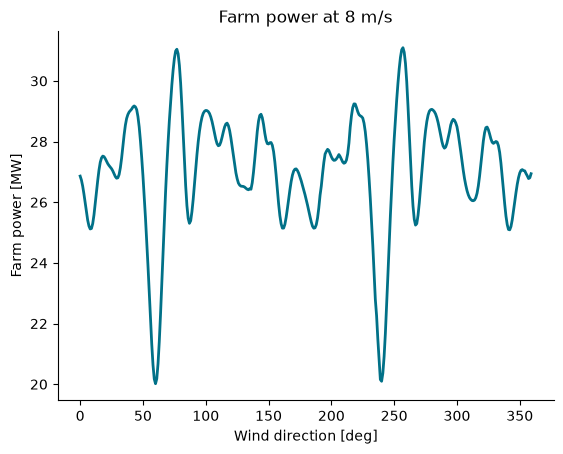

References¶

National Laboratory of the Rockies. (2025). FLORIS: Wake Modeling and Wind Farm Controls Software. Software, version 4. https://github.com/NatLabRockies/floris
Kainz, S., Quick, J., Souza de Alencar, M., Sanchez Perez Moreno, S., Dykes, K., Bay, C. J., Zaaijer, M. B., & Bortolotti, P. (2024). The IEA Wind 740-10-MW Reference Offshore Wind Plants [Techreport]. IEA Wind Task 55, National Laboratory of the Rockies. https://www.nlr.gov/docs/fy24osti/87923.pdf